Correlation, and regression analysis for curve fitting

The techniques described on this page are used to investigate relationships between two variables (x and y). Is a change in one of these variables associated with a change in the other? For example, if we increase the temperature do we increase the growth rate of a culture or the rate of a chemical reaction? Does an increase in DDT content of bird tissues correlate with thinning of the egg shell? Is an increase in slug density in a field plot associated with a decrease in seedling development?

We can use the technique of correlation to test the statistical significance of the association. In other cases we use regression analysis to describe the relationship precisely by means of an equation that has predictive value. We deal separately with these two types of analysis - correlation and regression - because they have different roles.

Correlation

Suppose that we took 7 mice and measured their body weight and their length from nose to tail. We obtained the following results and want to know if there is any relationship between the measured variables. [To keep the calculations simple, we will use small numbers]

Procedure

(1) Plot the results on graph paper. This is the essential first step, because only then can we see what the relationship might be - is it linear, logarithmic, sigmoid, etc?

In our case the relationship seems to be linear, so we will continue on that assumption. If it does not seem to be linear we might need to transform the data.

(2) Set out a table as follows and calculate S x, S y, S x², S y², S xy, and (mean of y).

	Weight (x)	Length (y)	x2	y2	xy
Mouse 1	1	2	1	4	2
Mouse 2	4	5	16	25	20
Mouse 3	3	8	9	64	24
Mouse 4	4	12	16	144	48
Mouse 5	8	14	64	196	112
Mouse 6	9	19	81	361	152
Mouse 7	8	22	64	484	176
Total	S x = 37	S y = 82	S x2 = 251	S y2 = 1278	S xy = 553
Mean	= 5.286	= 11.714

(3) Calculate = 55.429 in our case.

(4) Calculate = 317.429 in our case.

(5) Calculate (this can be positive or negative) = 119.571.

(6) Calculate r (correlation coefficient):

= 0.9014 in our case.

(7) Look up r in a table of correlation coefficients (ignoring + or - sign). The number of degrees of freedom is two less than the number of points on the graph (5 df in our example because we have 7 points). If our calculated r value exceeds the tabulated value at p = 0.05 then the correlation is significant. Our calculated value (0.9014) does exceed the tabulated value (0.754). It also exceeds the tabulated value for p = 0.01 but not for p = 0.001. If the null hypothesis were true (that there is no relationship between length and weight) we would have obtained a correlation coefficient as high as this in less than 1 in 100 times. So we can be confident that weight and length are positively correlated in our sample of mice.

Important notes:

1. If the calculated r value is positive (as in this case) then the slope will rise from left to right on the graph. As weight increases, so does the length. If the calculated value of r is negative the slope will fall from left to right. This would indicate that length decreases as weight increases.

2. The r value will always lie between -1 and +1. If you have an r value outside of this range you have made an error in the calculations.

3. Remember that a correlation does not necessarily demonstrate a causal relationship. A significant correlation only shows that two factors vary in a related way (positively or negatively). This is obvious in our example because there is no logical reason to think that weight influences the length of the animal (both factors are influenced by age or growth stage). But it can be easy to fall into the "causality trap" when looking at other types of correlation.

What does the correlation coefficient mean?

The part above the line in this equation is a measure of the degree to which x and y vary together (using the deviations d of each from the mean). The part below the line is a measure of the degree to which x and y vary separately.

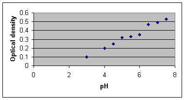
Regression analysis: fitting a line to the data

It would be tempting to try to fit a line to the data we have just analysed - producing an equation that shows the relationship, so that we might predict the body weight of mice by measuring their length, or vice-versa. The method for this is called linear regression.

However, this is not strictly valid because linear regression is based on a number of assumptions. In particular, one of the variables must be "fixed" experimentally and/or precisely measureable. So, the simple linear regression methods can be used only when we define some experimental variable (temperature, pH, dosage, etc.) and test the response of another variable to it.

The variable that we fix (or choose deliberately) is termed the independent variable. It is always plotted on the X axis. The other variable is termed the dependent variable and is plotted on the Y axis.

Suppose that we had the following results from an experiment in which we measured the growth of a cell culture (as optical density) at different pH levels.

We plot these results (see below) and they suggest a straight-line relationship.

Using the same procedures as for correlation, set out a table as follows and calculate S x, S y, S x², S y², S xy, and (mean of y).

	pH (x)	Optical density (y)	x2	y2	xy
	3	0.1	9	0.01	0.3
	4	0.2	16	0.04	0.8
	4.5	0.25	20.25	0.0625	1.125
	5	0.32	25	0.1024	1.6
	5.5	0.33	30.25	0.1089	1.815
	6	0.35	36	0.1225	2.1
	6.5	0.47	42.25	0.2209	3.055
	7	0.49	49	0.240	3.43
	7.5	0.53	56.25	0.281	3.975
Total	S x = 49	S y = 3.04	S x2 = 284	S y2 = 1.1882	S xy = 18.2
Mean	= 5.444	= 0.3378

Now calculate = 17.22 in our case.

Calculate = 0.1614 in our case.

Calculate (this can be positive or negative) = +1.649

Now we want to use regression analysis to find the line of best fit to the data. We have done nearly all the work for this in the calculations above.

The regression equation for y on x is: y = bx + a where b is the slope and a is the intercept (the point where the line crosses the y axis)

We calculate b as:

= 1.649 x 17.22 = 0.0958 in our case

We calculate a as:

a = - b

From the known values of (0.3378), (5.444) and b (0.0958) we thus find a (-0.1837).

So the equation for the line of best fit is: y = 0.096x - 0.184 (to 3 decimal places).

To draw the line through the data points, we substitute in this equation. For example:

when x = 4, y = 0.384, so one point on the line has the x,y coordinates (4, 0.384);

when x = 7, y = 0.488, so another point on the line has the x,y coordinates (7, 0.488).

It is also true that the line of best fit always passes through the point with coordinates , so we actually need only one other calculated point in order to draw a straight line.

Regression analysis using Microsoft Excel

Below is a printout of the Regression analysis from Microsoft "Excel". It is obtained simply by entering two columns of data (x and y) then clicking "Tools - Data analysis - Regression". We see that it gives us the correlation coefficient r (as "Multiple R"), the intercept and the slope of the line (seen as the "coefficient for pH" on the last line of the table). It also shows us the result of an Analysis of Variance (ANOVA) to calculate the significance of the regression (4.36 X 10^-7).

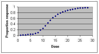
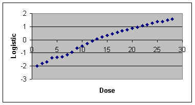
Presenting the results

The final graph should show:

(i) all measured data points;

(ii) the line of best fit;

(iii) the equation for the line;

(iv) the R² and p values.

Further applications: logarithmic and sigmoid curves

When we plot our initial results on a graph it will usually be clear whether they best fit a linear relationship or a logarithmic relationship or something else, like a sigmoid curve. We can analyse all these relationships in exactly the same way as above if we transform the x and y values as appropriate so that the relationship between x and y becomes linear. BEWARE - you MUST look at a scatter plot on graph paper to see what type of relationship you have. If you simply instruct a computer programme such as "Excel" to run a regression on untransformed data it will do this by assuming that the relationship is linear!

(i) For plots of data that suggest exponential (logarithmic) growth, convert all y values to log of y (using either log₁₀ or log_e). Then go through the linear regression procedures above, using the log y data instead of y data.

(ii) For sigmoid curves (drug dose response curves and UV killing curves are often sigmoid), the y values (proportion of the population responding to the treatment) can be converted using a logistic or probit transformation. Sometimes it is useful to convert the x (dose) data to logarithms; this condenses the x values, removing the long tails of non-responding individuals at the lowest and highest dose levels. A plot of logistic or probit (y) against dose (x) or log of dose (x) should show a straight-line relationship.

Converting between percentage, arcsin, logistic and probits in ‘Excel’

The table below shows part of a page from an ‘Excel’ worsksheet, produced as an exercise to show how transformations are performed. Columns in an Excel worksheet are headed A-F and rows are labelled 1-21, so each cell in the table can be identified (e.g. B2 or F11). Representative Proportions were inserted in cells A2-A21, and % values were inserted in cells B2-B21.

Then a formula was entered in cell C2 to convert Proportions to logistic values

The logistic transformation converts y to log(y/(1-y))

The formula (without spaces) entered into cell C2 was: =LOG(A2/(1-A2))

This formula is not seen in the cell, but as soon as we move out of cell C2 it automatically gives the logistic value (in C2) for the proportion in cell A2, seen in the printout below. Copying and then pasting this formula into every other cell of column C produces a corresponding logistic value (e.g. cell C3 contains the logistic value of the proportion in cell A3).

Similarly, a formula was entered in cell D2 to convert Percentage to Probit values.

The formula (without spaces) is: =NORMINV(B2/100,5,1) This was then pasted into all cells of column D

Next, a formula was entered in cell E2 to convert Probit to Percentage, and pasted into all cells of column E

The formula is: =NORMDIST(C2,5,1,TRUE)*100

The formula entered in cell F2 converts Percentage to Arcsine

The formula is: =ASIN(SQRT(A2/100))*180/PI()

The formula in cell G2 converts Arcsine to Percentage

The formula is: =SIN(E2/180*PI())^2*100

As an example of the use of transformations, the data from a fictitious dose-response curve (table below) are shown in two curves - first, without transformation and then after transforming the proportion responding to logistic values.

Dose Proportion Logistic 1 0.01 -1.99564 2 0.015 -1.81734 3 0.02 -1.6902 4 0.04 -1.38021 5 0.045 -1.32679 6 0.05 -1.27875 7 0.07 -1.12338 8 0.1 -0.95424 9 0.19 -0.62973 10 0.25 -0.47712 11 0.34 -0.28807 12 0.44 -0.10474 13 0.53 0.052178 14 0.62 0.212608 15 0.68 0.327359 16 0.74 0.454258 17 0.79 0.575408 18 0.83 0.688629 19 0.85 0.753328 20 0.88 0.865301 21 0.9 0.954243 22 0.92 1.060698 23 0.935 1.157898 24 0.95 1.278754 25 0.96 1.380211 26 0.96 1.380211 27 0.97 1.50965 28 0.975 1.591065